
Table of Contents
- Index Scan
- Index Only Scan (since PostgreSQL 9.2)
- Bitmap Index Scan / Bitmap Heap Scan / Recheck Cond
- Explain Analyze
- Example 1
- Example 2
- Takeaways
- References
- Next Steps
Index Scan
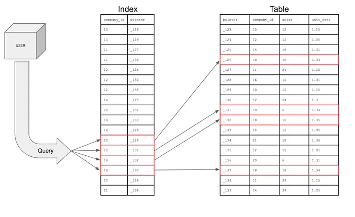
The index scan is one of the most fundamental access methods in PostgreSQL. Unlike a sequential scan that reads the entire table, an index scan leverages a pre-built index structure to efficiently locate specific rows.
How Index Scan Works
When PostgreSQL performs an index scan:
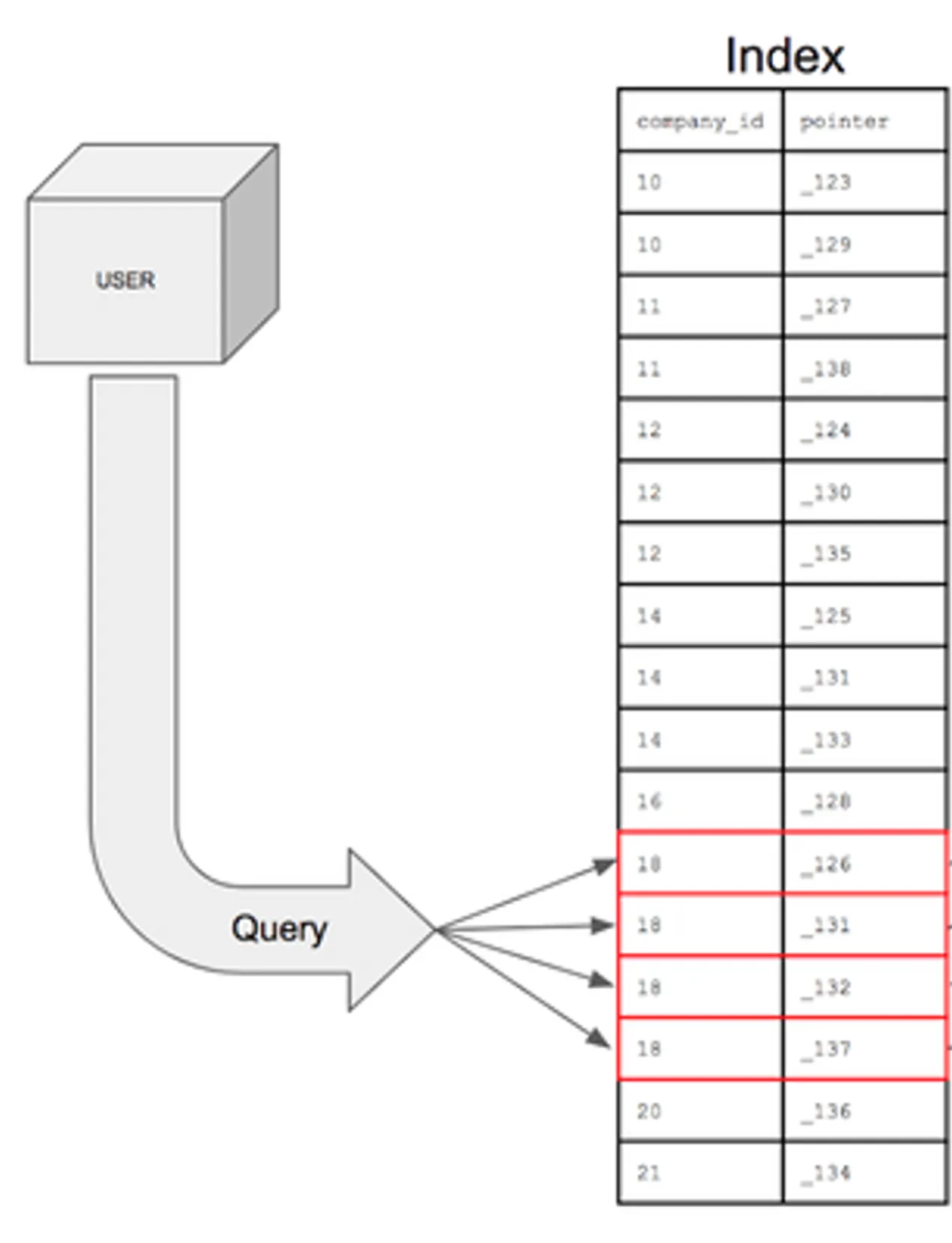
- It traverses the index structure (typically a B-tree) to find entries matching the query condition
- For each matching index entry, it retrieves the corresponding row’s physical location (TID - Tuple Identifier)
- It then visits the table to fetch the complete row data using these locations
Index scans are particularly efficient when:
- The query is highly selective (returning a small percentage of rows)
- The table is large
- The index covers the columns used in the WHERE clause
- The data needs to be returned in the index’s sort order
postgres=# explain select * from orders where id='45555'; QUERY PLAN--------------------------------------------------------------------------- Index Scan using orders_pkey on orders (cost=0.42..2.44 rows=1 width=27) Index Cond: (id = 45555)(2 rows)Note: Index scans can be less efficient than sequential scans when retrieving a large portion of the table, as each row access requires a random I/O operation to fetch the table data.
Index Only Scan (since PostgreSQL 9.2)
The Index Only Scan is a more specialized and optimized version of the index scan that can significantly improve query performance. Unlike a regular index scan that must access both the index and the table, an Index Only Scan retrieves all required data directly from the index itself, eliminating the need to visit the table.
How Index Only Scan Works
When PostgreSQL performs an Index Only Scan:
- It checks if all columns needed by the query are stored in the index
- It traverses the index structure to find matching entries
- It retrieves the required data directly from the index without accessing the table
This access method is particularly efficient when:
- The query only needs columns that are included in the index (either as key columns or included columns)
- The table is large, making table access expensive
- The visibility map indicates that all tuples are visible to all transactions (reducing the need for heap fetches)
postgres=# explain select id from orders where id='45555'; QUERY PLAN------------------------------------------------------------------------------- Index Only Scan using orders_pkey on orders (cost=0.42..1.44 rows=1 width=4) Index Cond: (id = 45555)(2 rows)Note: the select id above is the only column needed by the query, and it is included in the index.
Visibility Map Considerations (Advanced)
PostgreSQL maintains a visibility map to track which pages contain only tuples visible to all transactions. For an Index Only Scan to be truly index only, it needs to verify tuple visibility:
- If the visibility map shows all tuples on a page are visible, PostgreSQL can skip the heap check
- Otherwise, it must visit the heap to check visibility, reducing the efficiency advantage
Bitmap Index Scan / Bitmap Heap Scan / Recheck Cond
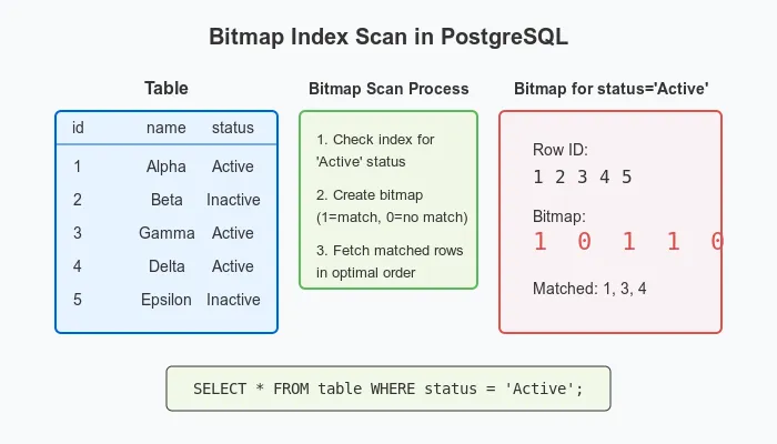
A Bitmap Index Scan is a sophisticated access method that PostgreSQL uses when an Index Scan would be inefficient but a Sequential Scan would be overkill. Here’s how it works:
How Bitmap Scans Work
- Gather Phase: The bitmap scan fetches all matching tuple-pointers (row locations) from the index in one operation
- Sort Phase: It organizes these pointers into a memory-efficient bitmap data structure, sorted by physical location on disk
- Access Phase: It then visits the table pages in physical order, minimizing random I/O operations
This approach combines the selectivity of indexes with the efficiency of sequential disk access patterns.
When Bitmap Scans Are Used
PostgreSQL typically chooses a bitmap scan when:
- The query is expected to return a moderate number of rows (too many for an efficient index scan)
- The rows are scattered throughout the table (making random access inefficient)
- Multiple indexes can be combined (using bitmap AND/OR operations)
Advantages of Bitmap Scans
- Reduced I/O: By sorting tuple accesses by physical location, it minimizes disk seek operations
- Index Combining: Can use multiple indexes simultaneously for complex conditions (e.g., WHERE x > 10 AND y < 20)
- Memory Efficiency: The bitmap structure uses minimal memory even for large result sets
- Batched Processing: Processes rows in batches, improving CPU cache utilization
postgres=# explain SELECT * FROM sampletable WHERE x < 423; QUERY PLAN----------------------------------------------------------------------------Bitmap Heap Scan on sampletable (cost=9313.62..68396.35 rows=402218 width=11) Recheck Cond: (x < '423'::numeric) -> Bitmap Index Scan on idx_x (cost=0.00..9213.07 rows=402218 width=0) Index Cond: (x < '423'::numeric)(4 rows)Explain Analyze
The Explain Analyze command provides a detailed breakdown of how PostgreSQL executes a query, including actual execution time and resource usage.
How Explain Analyze Works
The Explain Analyze command is used to get both the query plan and the actual execution time and resource usage.
- Execution Plan: It generates an execution plan similar to EXPLAIN
- Actual Execution: It actually executes the query and provides the actual execution time and resource usage.
!Caution: It actually executes the query.
postgres=# explain analyze select * from orders o, products p  where o.amount > 50000 and p.id=o.product_id;
                                                       QUERY PLAN------------------------------------------------------------------------------------------------------------------------- Hash Join  (cost=15.25..20507.79 rows=156593 width=50) (actual time=0.091..154.404 rows=157456 loops=1)   Hash Cond: (o.product_id = p.id)   ->  Seq Scan on orders o  (cost=0.00..20078.00 rows=156593 width=27) (actual time=0.006..128.617 rows=157456 loops=1)         Filter: (amount > '50000'::numeric)         Rows Removed by Filter: 842544   ->  Hash  (cost=9.00..9.00 rows=500 width=23) (actual time=0.080..0.081 rows=500 loops=1)         Buckets: 1024  Batches: 1  Memory Usage: 36kB         ->  Seq Scan on products p  (cost=0.00..9.00 rows=500 width=23) (actual time=0.004..0.039 rows=500 loops=1)
 Planning Time: 0.159 ms Execution Time: 158.574 ms
Let’s break down how to read and understand a query plan!
Reading Query Plans
When analyzing a query plan, focus on these key elements:
- Execution Time: The total time taken to complete the query
- Node Times: The actual processing time for each operation node
- Operation Types: The specific operations (like Seq Scan, Hash Join) being performed
- Node Hierarchy: How operations are nested and depend on each other
Query Plan Structure
Query plans in PostgreSQL follow a hierarchical structure:
- Each indented arrow (
->) represents a node in the execution tree - Child nodes are processed before their parent nodes
- The execution flows from the innermost (most indented) nodes outward
- Each node represents a specific operation PostgreSQL performs
Example 1
explain analyze select o.*, p.* from orders o, products p  where o.amount > 50000 and p.id=o.product_id;
                                                QUERY PLAN------------------------------------------------------------------------------------------------------------------------- Hash Join  (cost=15.25..20507.79 rows=156593 width=50) (actual time=0.094..154.278 rows=157456 loops=1)   Hash Cond: (o.product_id = p.id)   ->  Seq Scan on orders o  (cost=0.00..20078.00 rows=156593 width=27) (actual time=0.007..128.467 rows=157456 loops=1)         Filter: (amount > '50000'::numeric)         Rows Removed by Filter: 842544   ->  Hash  (cost=9.00..9.00 rows=500 width=23) (actual time=0.082..0.084 rows=500 loops=1)         Buckets: 1024  Batches: 1  Memory Usage: 36kB         ->  Seq Scan on products p  (cost=0.00..9.00 rows=500 width=23) (actual time=0.004..0.041 rows=500 loops=1) Planning Time: 0.203 ms Execution Time: 158.484 ms(10 rows)
Step-by-Step Breakdown of the Query Execution Plan
1. Sequential Scan (Seq Scan) on orders o
- The database performs a sequential scan on the orders table
- It applies the filter
amount > 50000, meaning it only keeps rows where the amount column exceeds 50,000 - Rows Processed:
- Total rows in orders: 1,000,000
- Rows matching the filter
(amount > 50000): 157,456 - Rows removed by the filter: 842,544 (remaining rows that didn’t satisfy the condition)
- This operation took 128.460 ms
2. Sequential Scan (Seq Scan) on products p
- The database scans the entire products table (500 rows)
- Since no filters are applied, all rows are read
- The database creates a hash table in memory using the
idcolumn as the key - This operation took 0.037 ms, and the hash table used 36 kB of memory
3. Hash Join (Hash Join) Between orders o and products p
- The database performs a hash join to match the product_id in orders with the id in products:
- The hash table (from products) allows quick lookups
- The database iterates through the filtered orders rows and checks for matches in the hash table
- The join condition is:
o.product_id = p.id
- Estimated output: 156,593 rows
- Actual output: 157,456 rows
- This operation took 154.278 ms
Final Output
- The database returns 157,456 rows, each containing all columns from both orders and products
- Total Execution Time: 158.484 ms
Example 2
Note: Only the where clause is different.
explain analyze select o.*, p.* from orders o, products p where o.amount > 99000 and p.id=o.product_id; QUERY PLAN---------------------------------------------------------------------------------------------------------------------------------- Nested Loop (cost=0.27..20274.89 rows=648 width=50) (actual time=0.062..119.781 rows=98 loops=1) -> Seq Scan on orders o (cost=0.00..20078.00 rows=648 width=27) (actual time=0.057..119.554 rows=98 loops=1) Filter: (amount > '99000'::numeric) Rows Removed by Filter: 999902 -> Index Scan using products_pkey on products p (cost=0.27..0.30 rows=1 width=23) (actual time=0.002..0.002 rows=1 loops=98) Index Cond: (id = o.product_id) Planning Time: 0.162 ms Execution Time: 119.804 ms(8 rows)Step-by-Step Breakdown of the Query Execution Plan
1. Sequential Scan (Seq Scan) on orders o
- The database scans the entire orders table.
- It applies the filter
amount > 99000, meaning it only keeps rows where amount is greater than 99,000. - Rows Processed:
- Total rows in orders: 1,000,000
- Rows matching the filter
(amount > 99000): 98 - Rows removed by the filter: 999,902
- Execution Time: 119.554 ms
2. Index Scan (Index Scan using products_pkey) on products p
- The database does NOT scan the entire products table.
- Instead, it uses the primary key index (products_pkey) to look up
id = o.product_id. - Why is an index scan used?
- The products table has an index on
id - Since we are retrieving a single row for each lookup.
- And the fact that the number of lookups is only 98, so index scan would be more efficient than a sequential scan.
- Execution Time: 0.002 ms per lookup.
- Total index scans performed: 98 (once for each matching row from orders).
- The products table has an index on
3. Nested Loop Join (Nested Loop)
- Since only 98 rows passed the filter from orders, the database chooses a Nested Loop Join instead of a Hash Join.
- How it works:
- The system takes one row from orders.
- It performs an index scan on products to find the matching row.
- It repeats this process 98 times.
- Total Execution Time: 119.781 ms.
Takeaways
- The query plan is a tree structure that shows the operations that PostgreSQL will perform to execute the query.
- Index scans are faster than sequential scans when retrieving a small percentage of rows.
- Index only scans are even faster than index scans when the query only needs columns that are included in the index.
- Bitmap scans are used when the query is expected to return a moderate number of rows.
- The Explain Analyze command provides a detailed breakdown of how PostgreSQL executes a query, including actual execution time and resource usage.
References
- How to read PostgreSQL query plan
- PostgreSQL EXPLAIN
- Explaining the Unexplainable
- PostgreSQL EXPLAIN ANALYZE
- How to read PostgreSQL query plan
Next Steps
- Learn about the different types of join strategies in PostgreSQL.
- Applying our learnings to optimize a real query.